Pico Technology Derek Hu

Abstract: Capturing and analyzing transient signal anomalies is a critical function of a modern oscilloscope. This article demonstrates three essential techniques in a PicoScope for this task: using persistence mode to visualize infrequent events, employing smart triggers to capture specific anomalies reliably, and applying Mask Limit Testing to automate pass/fail analysis. Through a practical walkthrough, you will learn a systematic workflow to isolate, capture, and diagnose irregularities in your waveforms.

1 Three typical methods for finding anomalies with a PicoScope

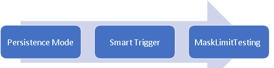
Figure 1 Three typical methods for finding anomalies with a PicoScope

Successfully isolating and analyzing signal anomalies is a fundamental challenge in electronics. PicoScope 7 software addresses this challenge with three powerful, complementary tools: Persistence Mode for visualization, Smart Trigger for precise capture, and Mask Limit Testing for automated validation

Persistence Mode provides an intuitive starting point. By superimposing thousands of waveform captures, it creates a density map that highlights transient anomalies against the normal signal. You can use the on-screen rulers to measure these visual glitches, runt pulses or anything else, gathering key parameters like amplitude and timing for your trigger setup afterwards. However, this mode has two primary limitations. First, it provides a composite image, not individual waveforms, preventing deep analysis with the scope’s full measurement and analysis suite. Second, it relies entirely on the instrument’s update rate. While PicoScope achieves an industry-leading rate of up to 300,000 waveforms per second, a single, ultrafast event can still slip between acquisitions.

For guaranteed capture, you must move to Smart Triggering. This method actively waits for a user-defined event—such as a pulse that is too narrow, a voltage that drops out of a window, or a specific logic pattern—and then captures the live waveform data surrounding it. Because triggering is a hardware function, it can capture events as short as a few nanoseconds. Crucially, every triggered capture is a complete digital waveform record, enabling full measurement, mathematical analysis, and saving. The inherent constraint is that a standard trigger isolates only one type of anomaly with each setting.

2 Capture anomalies with a PicoScope

2.1 Generate anomalies with built-in AWG in a PicoScope

PicoScope 3000E Series includes an integrated signal source, providing a convenient built-in stimulus for testing. All models feature a versatile function generator (FG) covering a frequency range from 100 µHz to 20 MHz, capable of outputting standard waveforms such as sine, square, triangle, DC voltage, ramp-up, ramp-down, sinc, Gaussian, and half-sine. Additionally, each unit is equipped with a 14-bit, 200 MS/s arbitrary waveform generator (AWG). Waveforms for the AWG can be created or edited directly in the PicoScope software, imported from oscilloscope traces, or loaded from spreadsheet files.

As shown in Figure 2, this setup leverages the built-in signal source. PicoScope 3000E’s FG/AWG output is connected directly to its own Channel A input via a BNC cable. The instrument is then controlled by PicoScope 7 software running on a laptop, connected via a standard USB interface. This creates a complete, self-contained test loop, ideal for demonstrating anomaly capture techniques.

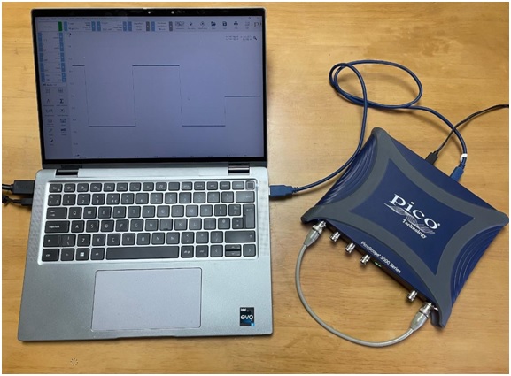
Figure 2 Test setup for generating signal anomalies with the built-in AWG in PicoScope 3418E

To generate a custom test signal containing anomalies, we configure the arbitrary waveform generator within PicoScope 7. The setup involves standard parameters like frequency, amplitude, and offset, along with the advanced tools in the AWG editor. As shown in Figure 3, you can draw a custom waveform or modify a standard one to include specific anomalies such as glitches or runt pulses.

Once the waveform is designed, clicking the Apply button in the top-left corner of the window commands the instrument to output the signal from its AWG port. This signal, which now contains the programmed anomalies, is fed directly into Channel A of the PicoScope via a BNC cable, creating a controlled signal path for demonstration and analysis.

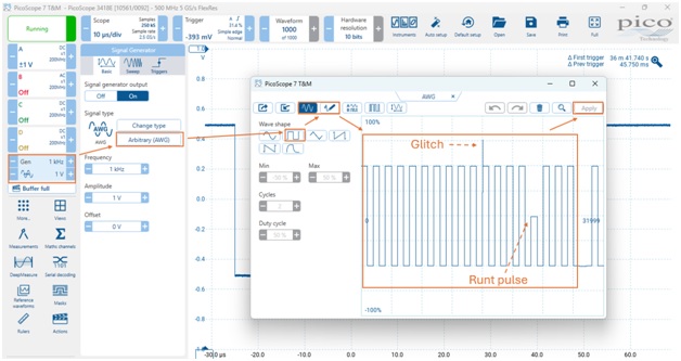
Figure 3 Configure built-in AWG in PicoScope 3418E to generate signal anomalies

The initial live signal on the screen appears unstable, with occasional anomalies—such as brief glitches—flickering in and out of view. To stabilize the display, we apply a basic edge trigger. This serves as the foundational first step, as we lack sufficient information about the anomaly’s specific characteristics (e.g., pulse width or amplitude) to configure a more advanced trigger at this stage. The setup for a basic edge trigger is shown in Figure 4.

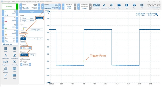
Figure 4 Stabilise the waveform display by using the basic edge trigger

2.2 Capture anomalies using Persistence Mode in PicoScope 7

Following the steps in Figure 5, select Persistence from the instrument toolbar. This will switch the display to Persistence Mode, where thousands of waveform acquisitions are superimposed. In this view, transient anomalies like glitches and runts become clearly visible against the main signal pattern.

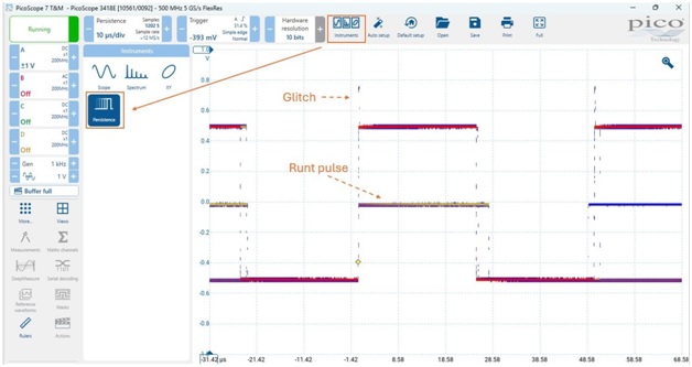
Figure 5 Capture anomalies using Persistence mode in PicoScope 7

As noted earlier, the persistence display provides a composite image rather than individual waveform data. Consequently, you can’t apply the full suite of PicoScope 7’s analysis tools, such as automated measurements or mathematical functions, to this specific view.

However, you can use the on-screen rulers—often referred to as cursors on traditional oscilloscopes—to perform basic manual measurements directly on the persistence image. Key parameters like the glitch amplitude and timing can be quantified in this way. This measured data then provides the precise information needed to configure a targeted Smart Trigger, allowing you to capture the anomaly as a standard, fully analyzable waveform.

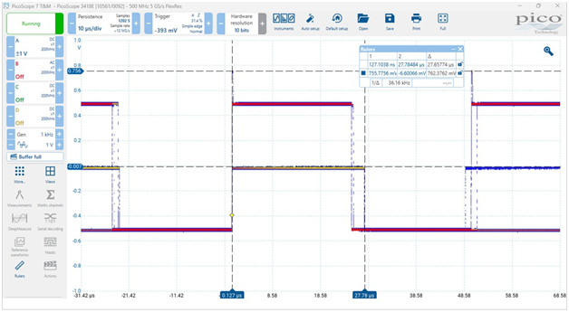
Figure 6 Make measurements with rulers under Persistent Mode

2.3 Capture anomalies with Smart Trigger in PicoScope 7

PicoScope 7 includes a wealth of standard Smart Triggers. To capture the glitch identified in Persistence mode, we can use a simple edge trigger. Based on the amplitude measurement from the persistence display, we position the trigger’s yellow threshold lozenge at the voltage level where the glitch occurs. This configures the scope to capture the precise moment the signal crosses that level, as shown in Figure 7.

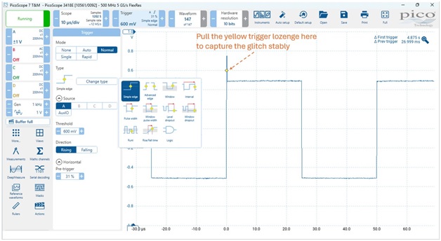
Figure 7 Capture the glitch with simple edge trigger in PicoScope 7

Similarly, a Runt Trigger can be configured to capture the runt pulse identified earlier. As illustrated in Figure 8, this trigger condition is activated when a pulse crosses one threshold but fails to cross the other, meaning its amplitude remains between the defined upper and lower voltage levels.

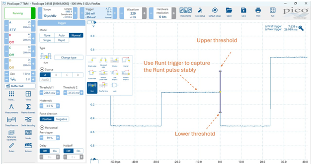
Figure 8 Capture the Runt pulse with Runt trigger in PicoScope 7

Once the anomaly is captured as a standard waveform, the full power of PicoScope 7 becomes available. You can now apply any function or measurement tool for detailed analysis. As shown in Figure 9, this includes both manual measurements using the on-screen rulers and automated measurements via the built-in measurement suite.

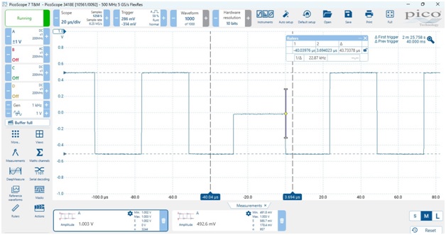
Figure 9 Capture the Runt pulse with Runt Trigger in PicoScope 7

2.4 Capture anomalies with Mask Limit Testing in PicoScope 7

Mask Limit Testing automates the capture of all waveform deviations by consecutively comparing live signals against a known good reference. To use it, first capture a good signal. The software can then automatically generate a pass/fail mask around this reference waveform. Once active, Mask Limit Testing monitors the signal in real-time, instantly capturing and saving any waveform segment that violates the mask. This allows multiple, diverse anomalies to be isolated in a single configuration.

As shown in Figure 10, you can automatically generate a mask for a good waveform under test. Following this process creates a precise tolerance envelope, enabling efficient long-term validation and fault detection.

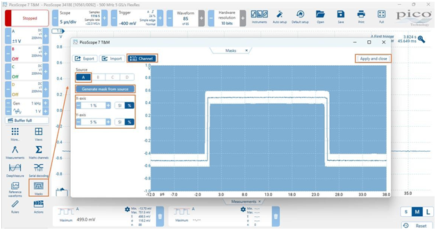
Figure 10 Generate a mask on a good signal in PicoScope 7

Figure 11 demonstrates the result. Both the glitch and runt anomalies are captured simultaneously in a single configuration. Furthermore, the Mask Limit Testing provides immediate analytical feedback. The statistics panel at the bottom of the screen shows, for example, that the scope captured 104 waveforms during the test, of which five were flagged for mask violations.

All captured waveforms are stored in the instrument’s buffer. You can quickly filter this buffer to isolate and review only the waveforms that violated the mask. Crucially, because Mask Limit Testing captures standard digital waveform data, you can apply the full suite of PicoScope 7’s measurement and analysis tools to these saved captures for detailed investigation as well.

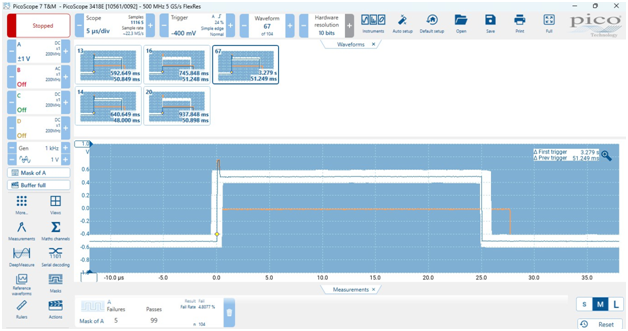
Figure 11 Capture, locate and analyze all anomalies with Mask Limit Testing in PicoScope 7

3 Conclusions

Successfully capturing and diagnosing signal anomalies requires a methodical approach that evolves from visualization to precise, automated capture. As demonstrated, PicoScope provides a powerful, integrated workflow for this entire process. Persistence Mode serves as the essential first step, offering a visual map to reveal the presence and basic characteristics of elusive events. The quantitative data got from this view directly supports the setup of a Smart Trigger—such as Edge, Pulse Width, or Runt—which isolates a specific anomaly from lots of acquisitions as a fully analyzable waveform.

For the most complex debugging and validation tasks, Mask Limit Testing delivers unparalleled efficiency. By automatically capturing any deviation from a known good signal, it enables comprehensive, unattended monitoring to catch intermittent and multiple fault types with a single test setup.

Together, these three tools—Persistence Mode, Smart Triggering, and Mask Limit Testing—form a complete hierarchy of signal anomalies catching and analyzing within PicoScope 7. By using them, you can observe a problem simply, capturing it reliably and analyzing it in depth, dramatically accelerating the debugging in electronic design.